Designing an efficient A-weighting filter
A-weighting is often used when measuring sound pressure (i.e. loudness) to make a recorded audio clip more representative of what would be perceived by the human ear. It works by increasing or decreasing the magnitude of audio frequencies according to what humans can hear. This leads to the A-weighted measurement of decibels (dBA) which is used to quantify how loud something is.
This was essential to a recent project of mine, the NoiseCard, which measures ambient noise levels to inform the user about the auditory safety of their surroundings. The NoiseCard runs off of just a few milliwatts of power which was made possible by slowing down its processor and minimizing the amount of audio samples that run through the frequency-weighting calculations. These calculations involve five stages of IIR filters: two that flatten the microphone's specific frequency response and three that apply the A-weighting.
The microcontroller is an STM32G031J8, a Cortex-M0+ core with no floating-point hardware. Running at just 16MHz as well (to save power; its max speed is 64MHz), the STM32 is limited to processing just 16 samples per each 256-sample block that is recorded by the microphone. A Cortex-M4F core would have been a better choice for these computations, but my goal is to keep the cost of the NoiseCard low and maximize the performance that I can get out of this microcontroller.
In this writeup, I'm going to try and design a more efficient A-weighting algorithm that could allow the NoiseCard to process more of the samples that it records. This will lead to either higher power efficiency and/or a more accurate measurement of dBA.
Filter design
To start, I had to remember what university taught me about IIR filtering years ago. Lacking in this recall, I turned to Python and this GitHub repo to make a quick A-weighting plot. A scipy library is used that easily generates IIR filters based on specifications like frequency, order, etc; we'll rely on this support pretty heavily:
# Create our X axis values, the frequencies to test at:
gs = 2 * math.pi * numpy.geomspace(10, 24000, 1000)

z, p, k = A_weighting(48000, output='zpk')
_, hA = signal.freqz_zpk(z, p, k, gs, fs=48000)
plt.semilogx(gs, 20 * numpy.log10(hA), label='A')
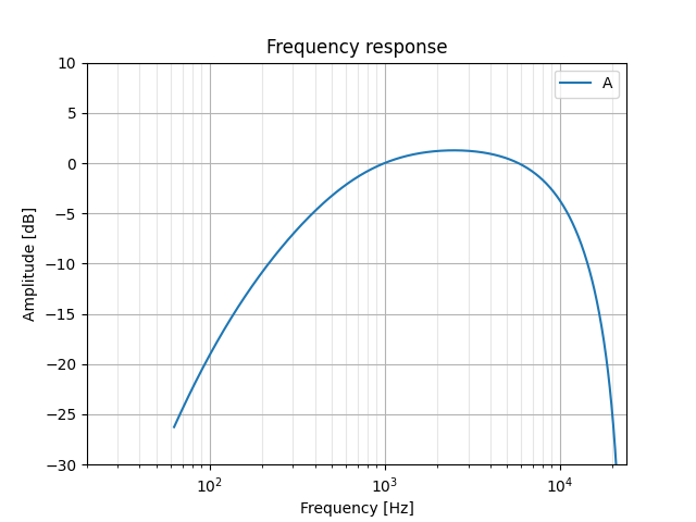
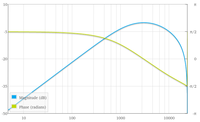
I do recognize this curve as kind of a band-pass filter, though its slopes are of varying steepness. A band-pass can be implemented as a second-order IIR filter; using this online calculator to plot one gave me a promising start:
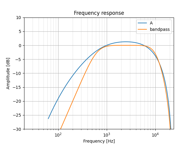
Our Python-equivalent would be scipy.signal.iirfilter which I've tried out below. A few things are off though:
- The filter's gain does not exceed zero
- The slope of the low frequency response is too steep
- The slope of the high frequency response is not as "round" as the A-weighting
z, p, k = signal.iirfilter(2, [600, 10000], btype='bandpass', analog=False, fs=48000, output='zpk')
_, hB = signal.freqz_zpk(z, p, k, gs, fs=48000)
plt.semilogx(gs, 20 * numpy.log10(hB), label='bandpass')
We'll do two things to fix this up a bit: first, increase the filter's gain by multiplying its k factor (zpk means zeros, poles, and gain); second, we'll reduce the response's slope by telling iirfilter to make this a first-order filter (though I'm pretty sure a bandpass can't be of order 1...). Finally, we'll also tweak the critical frequencies a bit:
z, p, k = signal.iirfilter(1, [600, 8500], btype='bandpass', analog=False, fs=48000, output='zpk')
k = k * 1.145
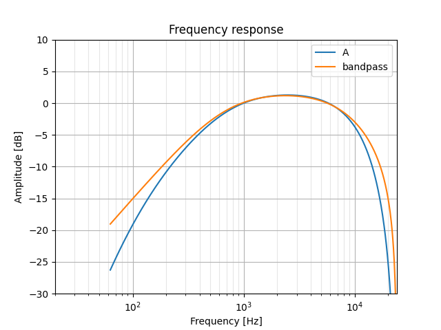
Now our filter's slopes are too soft... since these are determined by the whole-number order of the filter, we're going to need to tack on additional filter stages to get finer control over this. We'll try using some first-order low- and high-pass filters; ideally, these will be easy to implement and won't significantly increase our final processing time.
Low-pass filter
A first-order low-pass filter should help attenuate our band-pass filter's high-frequency response. I ended up choosing a cut-off frequency of 12kHz:
z, p, k = signal.iirfilter(1, 12000, btype='lowpass', analog=False, fs=48000, output='zpk')
_, hL = signal.freqz_zpk(z, p, k, gs, fs=48000)
plt.semilogx(gs, 20 * numpy.log10(hL), label='lowpass')
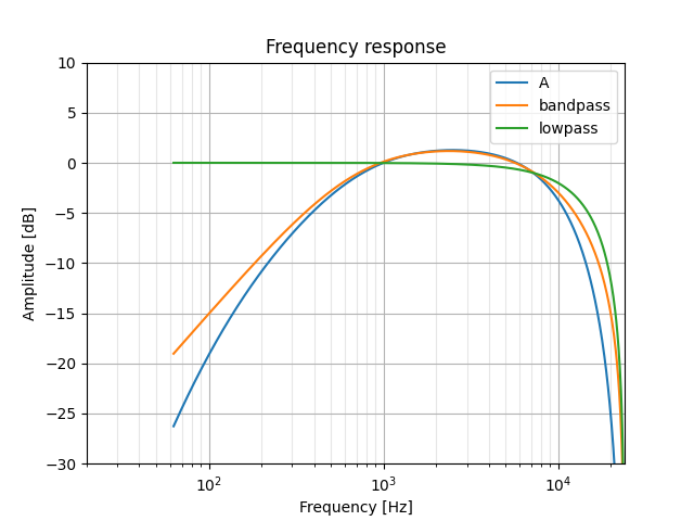
Looks like the sum of the band-pass and low-pass responses should get us what we want. In our script, we can create our multi-filter response by multiplying the outputs of freqz_zpk together; on the microcontroller, we'll just pass the output of one filter into the next.
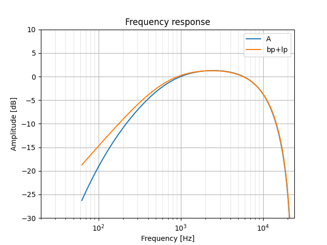
I've also gone ahead here and adjusted the band-pass parameters to make this two-filter response line up with A-weighting as much as possible.
z, p, k = signal.iirfilter(1, [600, 10000], btype='bandpass', analog=False, fs=48000, output='zpk')
k = k * 1.17
_, hB = signal.freqz_zpk(z, p, k, gs, fs=48000)

...

plt.semilogx(gs, 20 * numpy.log10(hB * hL), label='bp+lp')
High-pass filter
The results we just saw are pretty promising. We'll add a third (and hopefully final) filter now: a high-pass that will bring down our low-frequency response.
z, p, k = signal.iirfilter(1, 145, btype='highpass', analog=False, fs=48000, output='zpk')
_, hH = signal.freqz_zpk(z, p, k, gs, fs=48000)

plt.semilogx(gs, 20 * numpy.log10(hH), label='highpass')
plt.semilogx(gs, 20 * numpy.log10(hB * hL * hH), label='bp+lp+hp')
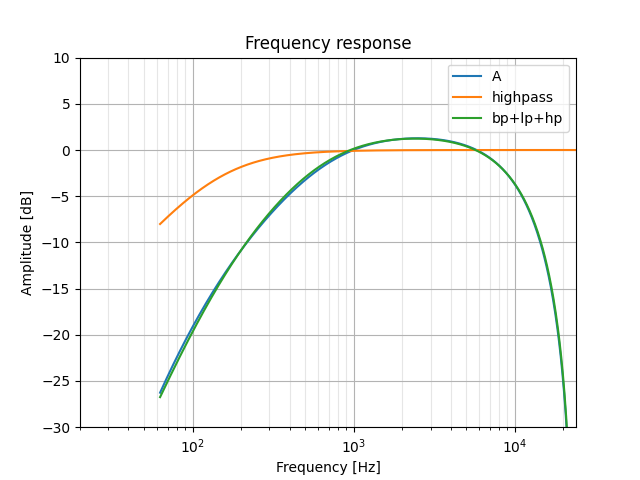
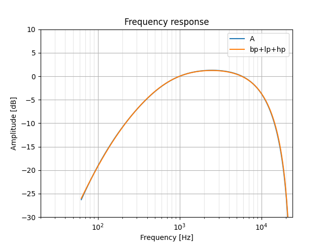
Looks like we've got this down! If we bump the band-pass filter's lower frequency up to 640Hz and bring the high-pass cut-off down to 120Hz, we end up with what is a pretty great match (at least, good enough for me):
Getting the coefficients
Now it's time to get this filter into code. The NoiseCard's firmware is written in C++, but what we write here will be indistinguishable from C so I'll just call it "C/C++".
For this implementation, we'll need to get the coefficients of each filter stage in some form that we can work with. A common way to go about this is with second-order sections (SOSs) which have five significant values: a0, a1, a2, b1, and b2. Using this handy code, we can apply an SOS like so:
float process(float in) {
    float out = in * a0 + z1;
    z1 = in * a1 + z2 - b1 * out;
    z2 = in * a2 - b2 * out;
    return out;
}
Our coefficients are discovered by calling scipy.signal.zpk2sos and printing the output:
band pass: [0.48290116  0.          -0.48290116  1.  -1.10133498  0.17452794]
 low pass: [0.5         0.5          0.          1.  -5.5511e-17  0.        ]
high pass: [0.99220706 -0.99220706   0.          1.  -0.98441413  0.        ]
(the fourth column of 1's are the b0 coefficients which aren't important to us)
We could just plug these numbers into process() and call it a day, but I think we would have a much better time optimizing if we could round some of these numbers to more convenient values... how would that look?
scipy.signal.sosfreqz lets us plot a frequency response based on SOSs:
sos = [[ 0.5,  0,   -0.5,  1, -1.10133498,  0.17452794],
       [ 0.5,  0.5   0,    1,  0,           0         ],
       [ 1.0, -1.0   0,    1, -0.98441413,  0         ]]
wS, hS = signal.sosfreqz(sos, fs=48000)
plt.semilogx(wS, 20 * numpy.log10(hS), label='sos')
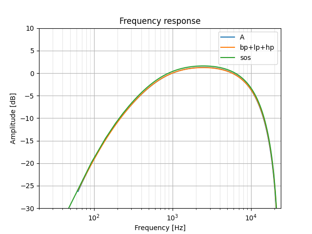
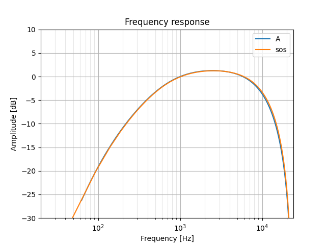
Not bad! A few more adjustments via some trial-and-error, and we have a much nicer filter to work with:
sos = [[ 0.5,  0,   -0.5,  1, -1.062,  0.14],
       [ 0.5,  0.5,  0,    1,  0,      0   ],
       [ 1.0, -1.0,  0,    1, -0.985,  0   ]]
C/C++ implementation
Let's start by copying out our process() function to work through our three filter stages. Our input/output pairs will be in/out1, out1/out2, and out2/out3 with out3 being the filter's final result.
We'll also rename the z variables accordingly and substitute in the filter coefficients:
float process(float in) {
    static float z1 = 0, z2 = 0, z3 = 0, z4 = 0, z5 = 0, z6 = 0;

    float out1 = in * 0.5f + z1;
    z1 = in * 0 + z2 - -1.062f * out1;
    z2 = in * -0.5f - 0.14f * out1;

    float out2 = out1 * 0.5f + z3;
    z3 = out1 * 0.5f + z4 - 0 * out2;
    z4 = out1 * 0 - 0 * out2;

    float out3 = out2 * 1 + z5;
    z5 = out2 * -1 + z6 - -0.985f * out3;
    z6 = out2 * 0 - 0 * out3;

    return out3;
}
Right away we see multiplications by zero that we can cut out. This eliminates two of our z state variables as well:
float process(float in) {
    static float z1 = 0, z2 = 0, z3 = 0, z5 = 0;

    float out1 = in * 0.5f + z1;
    z1 = z2 + 1.062f * out1;
    z2 = in * -0.5f - 0.14f * out1;

    float out2 = out1 * 0.5f + z3;
    z3 = out1 * 0.5f;

    float out3 = out2 + z5;
    z5 = -out2 + 0.985f * out3;

    return out3;
}
Next, I'm going to do some factoring to remove as many multiplications as I can. It's worth noting that negating is distinct from multiplying by -1 in our case: negation can be implemented by simply toggling the "sign" bit of the given floating-point number.
Factoring 0.5f out of the second stage turns out2 into a single addition. Balancing that is multiplications by 2.f in the first stage, which won't impact run-time since they can simply be incorporated into the existing coefficients:
float out1 = 0.5f * 0.5f * in + 0.5f * z1;
z1 = z2 + 1.062f * 2.f * out1;
z2 = in * -0.5f - 0.14f * 2.f * out1;

float out2 = out1 + z3;
z3 = out1;
We can save a multiplication if we also factor out 0.5f from in...
in *= 0.5f;

float out1 = 0.5f * in + 0.5f * z1;
z1 = z2 + 1.062f * 2.f * out1;
z2 = -1.f * in - 0.14f * 2.f * out1;
In fact, we'll do this twice. Reason #1 is that the incoming microphone samples (received via I2S) are left-aligned; they require a right bitwise shift before they can be used, so if we just shift by two more bits (an equivalent to dividing by 4) then we'll have done this multiplication for free!
//in *= 0.25f; // Assume input will already be divided by 4

float out1 = in + 0.5f * z1;
z1 = z2 + 1.062f * 2.f * out1;
z2 = -2.f * in - 0.14f * 2.f * out1;
Finally, we can actually cancel out all of the 0.5f and 2.f factors in this first stage. Factor 2.f out of z2, then 2.f out of z1, and use that to cancel the 0.5f in out1.
The result? An A-weighting algorithm that uses just a few multiply-adds and additions:
float process(float in_div4) {
    static float z1 = 0, z2 = 0, z3 = 0, z5 = 0;

    float out1 = in_div4 + z1;
    z1 = 1.062f * out1 + z2;
    z2 = -0.14f * out1 - in_div4;

    float out2 = out1 + z3;
    z3 = out1;

    float out3 = out2 + z5;
    z5 = 0.985f * out3 - out2;

    return out3;
}
I do like hardware floating-point units
I developed these optimizations on Compiler Explorer, watching the dissassembly of the function compiled for ARM Cortex-M4F. The floating-point unit (FPU) provides multiply-adds, multiply-subtracts, and much more as single processor instructions.
With optimizations enabled, this packs the entire algorithm into just 20 instructions:
process(float):
        ldr     r3, .L3
        vldr.32 s14, .L3+4
        vldr.32 s13, [r3]
        vldr.32 s15, [r3, #8]
        vldr.32 s12, [r3, #12]
        vldr.32 s11, [r3, #4]
        vldr.32 s9, .L3+8
        vldr.32 s10, .L3+12
        vadd.f32        s13, s0, s13
        vadd.f32        s15, s13, s15
        vfma.f32        s11, s13, s14
        vadd.f32        s12, s15, s12
        vmov.f32        s14, s0
        vfnms.f32       s14, s13, s9
        vfnms.f32       s15, s12, s10
        vstr.32 s13, [r3, #8]
        vstr.32 s11, [r3]
        vstr.32 s14, [r3, #4]
        vstr.32 s15, [r3, #12]
        vmov.f32        s0, s12
        bx      lr
.L3:
        .word   .LANCHOR0
        .word   1065873310
        .word   -1106289623
        .word   1065101558
On our poor Cortex-M0+ though, we need to make do with a software floating-point implementation. NoiseCard uses Qfplib-M0-full, which gives us addition in 76 cycles and multiplication in 62 cycles.
Here's the optimized assembly for the M0+. Let's use our Qfplib numbers for the __aeabi calls and estimate the other instructions:
process(float):
        push    {r4, r5, r6, lr} ; 1 + 4 cycles
        ldr     r4, .L3          ; ldr, adds, and str will be single-cycle
        adds    r6, r0, #0
        ldr     r1, [r4]
        bl      __aeabi_fadd     ; +2 cycles for the branch and return
        ldr     r1, .L3+4
        adds    r5, r0, #0
        bl      __aeabi_fmul
        ldr     r1, [r4, #4]
        bl      __aeabi_fadd
        ldr     r1, .L3+8
        str     r0, [r4]
        adds    r0, r5, #0
        bl      __aeabi_fmul
        adds    r1, r6, #0
        bl      __aeabi_fsub
        ldr     r1, [r4, #8]
        str     r0, [r4, #4]
        adds    r0, r5, #0
        bl      __aeabi_fadd
        ldr     r1, [r4, #12]
        str     r5, [r4, #8]
        adds    r6, r0, #0
        bl      __aeabi_fadd
        ldr     r1, .L3+12
        adds    r5, r0, #0
        bl      __aeabi_fmul
        adds    r1, r6, #0
        bl      __aeabi_fsub
        str     r0, [r4, #12]
        adds    r0, r5, #0
        pop     {r4, r5, r6, pc} ; 3 + 4 cycles
My rough calculations total this up to 693 cycles. What does that get us?
- The NoiseCard's I2S interrupt fires every 512 samples at a sampling rate of 48kHz, so the interrupt routine we process from needs to complete in under
512/48000 = 10.666milliseconds. - Running at 16MHz, that means we can process up to around
.010666 * 16e6 / 693 = 246samples! - ...but, we also need to transform the I2S data from two channels of
uint32_ts to a single channel offloats (including that right shift we talked about earlier) :( - and we need to accumulate the sum of squares for the filtered samples to eventually get a dBA value.
In my tests, I was only able to process the entire 256-sample block if I pushed the microcontroller's clock speed up to 64MHz. Using a GPIO to signal the entry and exit of the interrupt routine suggests that it's taking around 80% of that 10.666ms window to execute. In terms of average power consumption, this led to an increase from ~3 milliwatts to ~10mW. That's still relatively little power for accurate dBA monitoring; in my opinion, it's a success.
The previous implementation
I originally worked off of code from this project for A-weighting and SOS filtering. Its A-weighting filter also consists of three stages, though it uses a full set of precise coefficients as well as an explicit gain factor:
SOS_IIR_Filter A_weighting = {
  /* gain: */ sos_t(0.169994948147430f),
  /* sos: */ { // Second-Order Sections {b1, b2, -a1, -a2}
    { sos_t(-2.00026996133106f),  sos_t(+1.00027056142719f),
      sos_t(-1.060868438509278f), sos_t(-0.163987445885926f) },
    { sos_t(+4.35912384203144f),  sos_t(+3.09120265783884f),
      sos_t(+1.208419926363593f), sos_t(-0.273166998428332f) },
    { sos_t(-0.70930303489759f),  sos_t(-0.29071868393580f),
      sos_t(+1.982242159753048f), sos_t(-0.982298594928989f) } }
};
For each filter stage, a loop like below is run. Each stage's delay state is accessed via ww.
Note that the sum_sqr line only appears for final filter (output) stage.
for (auto& s : samples) {
    auto f6 = s + coeffs.a1 * ww.w0 + coeffs.a2 * ww.w1;
    s = f6 + coeffs.b1 * ww.w0 + coeffs.b2 * ww.w1;
    ww.w1 = std::exchange(ww.w0, f6);
    sum_sqr += s * gain * s * gain;
}
So, this code was iterating over the entire sample data three separate times while also executing additional multiplications for its coefficients and gain. Our newly designed filter will give us quite the boost in efficiency -- I hope others might find it useful too.
You can get the Python script and C function from here.
